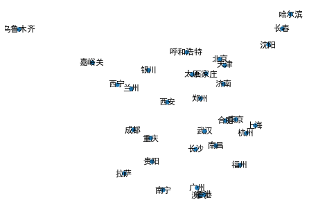
defget_city_info(city_coordination): city_location = {} first = True for line in city_coordination.split('\n'): if line.startswith('//'): continue if line.strip()=="":continue city =re.findall("name:'(\w+)'",line)[0] x_y = re.findall("Coord:\[(\d+.\d+),\s(\d+.\d+)\]",line)[0] if first ==True: print("x_y: ",x_y) x_y = tuple(map(float,x_y)) city_location[city] = x_y if first ==True: print("city:",city ) print("x_y: ",x_y) first =False return city_location
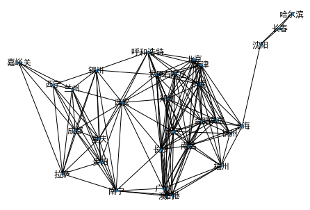
Build connection between. Let’s assume that two cities are connected if their distance is less than 700km
1
threshold = 700# defined the threshold
1
from collections import defaultdict
1 2 3 4 5 6 7 8 9 10 11 12
defbuild_connection(city_info): cities_connection = defaultdict(list) cities = list(city_info.keys()) for c1 in cities: for c2 in cities: if c1 == c2 : continue if get_city_distance(c1,c2) < threshold: cities_connection[c1].append(c2) return cities_connection
defsearch_2(graph,start,destination,search_strategy): pathes = [[start]] visited =set() # ! while pathes: path = pathes.pop(0) froniter =path[-1] if froniter in visited:continue# ! if froniter == destination: return path successors = graph[froniter] for city in successors: if city in path:continue#check loop new_path = path + [city] pathes.append(new_path) pathes =search_strategy(pathes) visited.add(froniter) # ! #
1 2 3 4 5 6 7
defsort_by_distance(pathes): defget_distance_of_path(path): distance = 0 for i,_ in enumerate(path[:-1]): distance += get_city_distance(path[i],path[i+1]) return distance return sorted(pathes,key =get_distance_of_path)
1
2
3
4
5
defget_distance_of_path(path): distance = 0 for i,_ in enumerate(path[:-1]): distance += get_city_distance(path[i],path[i+1]) return distance
".. _boston_dataset:\n\nBoston house prices dataset\n---------------------------\n\n**Data Set Characteristics:** \n\n :Number of Instances: 506 \n\n :Number of Attributes: 13 numeric/categorical predictive. Median Value (attribute 14) is usually the target.\n\n :Attribute Information (in order):\n - CRIM per capita crime rate by town\n - ZN proportion of residential land zoned for lots over 25,000 sq.ft.\n - INDUS proportion of non-retail business acres per town\n - CHAS Charles River dummy variable (= 1 if tract bounds river; 0 otherwise)\n - NOX nitric oxides concentration (parts per 10 million)\n - RM average number of rooms per dwelling\n - AGE proportion of owner-occupied units built prior to 1940\n - DIS weighted distances to five Boston employment centres\n - RAD index of accessibility to radial highways\n - TAX full-value property-tax rate per $10,000\n - PTRATIO pupil-teacher ratio by town\n - B 1000(Bk - 0.63)^2 where Bk is the proportion of blacks by town\n - LSTAT % lower status of the population\n - MEDV Median value of owner-occupied homes in $1000's\n\n :Missing Attribute Values: None\n\n :Creator: Harrison, D. and Rubinfeld, D.L.\n\nThis is a copy of UCI ML housing dataset.\nhttps://archive.ics.uci.edu/ml/machine-learning-databases/housing/\n\n\nThis dataset was taken from the StatLib library which is maintained at Carnegie Mellon University.\n\nThe Boston house-price data of Harrison, D. and Rubinfeld, D.L. 'Hedonic\nprices and the demand for clean air', J. Environ. Economics & Management,\nvol.5, 81-102, 1978. Used in Belsley, Kuh & Welsch, 'Regression diagnostics\n...', Wiley, 1980. N.B. Various transformations are used in the table on\npages 244-261 of the latter.\n\nThe Boston house-price data has been used in many machine learning papers that address regression\nproblems. \n \n.. topic:: References\n\n - Belsley, Kuh & Welsch, 'Regression diagnostics: Identifying Influential Data and Sources of Collinearity', Wiley, 1980. 244-261.\n - Quinlan,R. (1993). Combining Instance-Based and Model-Based Learning. In Proceedings on the Tenth International Conference of Machine Learning, 236-243, University of Massachusetts, Amherst. Morgan Kaufmann.\n"
1
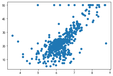
X_rm = x[:,5]
1
2
# plot the RM with respect to y plt.scatter(X_rm,y)
<matplotlib.collections.PathCollection at 0x11955a9f148>
Gradient descent
Assume that the target function is a linear function
1 2 3
# define target function defprice(rm,k,b): return k*rm + b
Define mean square loss
1 2 3
# define loss function defloss(y,y_hat): return sum((y_i - y_hat_i)**2for y_i,y_hat_i in zip(list(y),list(y_hat)))/len(list(y))
Define partial derivatives
1 2 3 4 5 6 7 8 9 10 11 12 13 14
#define partial derivative defpartial_derivative_k(x,y,y_hat): n = len(y) gradient = 0 for x_i,y_i,y_hat_i in zip(list(x),list(y),list(y_hat)): gradient += (y_i - y_hat_i) * x_i return-2/n * gradient
defpartial_derivative_b(y,y_hat): n =len(y) gradient = 0 for y_i,y_hat_i in zip(list(y),list(y_hat)): gradient+= (y_i-y_hat_i) return-2/n* gradient
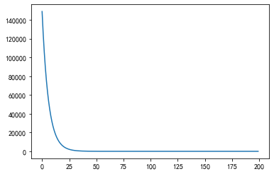
iteration_num =200 losses = [] for i in range(iteration_num): price_use_current_parameters = [price(r,k,b) for r in X_rm] # \hat{y} current_loss = loss(y,price_use_current_parameters) losses.append(current_loss) #print("Iteration {},the loss is {},parameters k is {} and b is {}".format(i,current_loss,k,b)) k_gradient = partial_derivative_k(X_rm,y,price_use_current_parameters) b_gradient = partial_derivative_b(y,price_use_current_parameters) k = k + (-1 * k_gradient) * learning_rate b = b + (-1 * b_gradient) * learning_rate
best_k =k best_b =b print("best_k is{},best_b is {}".format(best_k,best_b))
best_k is12.41253129958806,best_b is -55.72859329657179
1
plt.plot(list(range(iteration_num)),losses)
[<matplotlib.lines.Line2D at 0x119550b6fc8>]
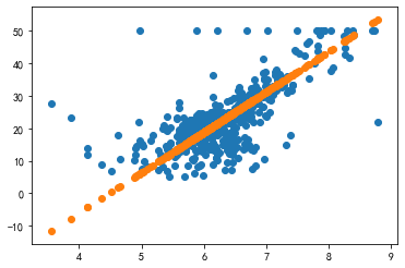
1 2 3 4
price_use_best_paramters = [price(r,best_k,best_b) for r in X_rm]